Ideal Beam-Splitter Example

This example demonstrates the use of the BeamSplitter model, we also make use of NumberStateSource to generate the state.

from __future__ import annotations
import numpy as np
from symop.devices.models import BeamSplitter, NumberStateSource
from symop.devices.models.detectors.number_detector import NumberDetector
from symop.modes.labels import Path, Polarization
from symop.modes.envelopes import GaussianEnvelope
from symop.polynomial.state.ket import KetPolyState

# Visualization Package
import symop.viz as VI

Setup

Set up mode labels for sources and beamsplitter (50/50)

src_a = NumberStateSource(
    envelope=GaussianEnvelope(omega0=100.0, sigma=50.0, tau=0.0),
    polarization=Polarization.H(),
    n=1,
)

src_b = NumberStateSource(
    envelope=GaussianEnvelope(omega0=100.0, sigma=50.0, tau=0.0),
    polarization=Polarization.H(),
    n=1,
)

bs = BeamSplitter(theta=np.pi / 4, phi_r=0)

1) Generate the states

• Generate vacuum states for the sources to populate

vac = KetPolyState.vacuum()

state_a = src_a(vac, ports={"out": Path("src_a_out")}).with_label("in_A")
state_b = src_b(vac, ports={"out": Path("src_b_out")}).with_label("in_B")

2) Interfere the two states

• Join the states

• Interfere them

state_joint = state_a.join(state_b).with_label("joint")

state_interfered = bs(
    state_joint,
    ports={
        "in0": Path("src_a_out"),
        "in1": Path("src_b_out"),
        "out0": Path("bs_out0"),
        "out1": Path("bs_out1"),
    },
).with_label("interfered")

2a) Inspect the states

VI.display_many(state_a, state_b, state_joint, state_interfered)

Why does the output contain several terms?

The beamsplitter acts linearly on each input creation operator. Since the joint input state contains one photon in each input path, the output is obtained by expanding the product of two linear combinations of output-mode operators.

This produces amplitudes for all possible two-photon output configurations:

• both photons in output path 0,

• one photon in each output path,

• both photons in output path 1.

These terms are amplitudes, not measurement probabilities. The actual detection statistics depend on the overlaps between the output modes. When the two inputs are fully indistinguishable (same envelope and same polarization), interference can cancel coincidence contributions and enhance bunching, as in the Hong-Ou-Mandel effect.

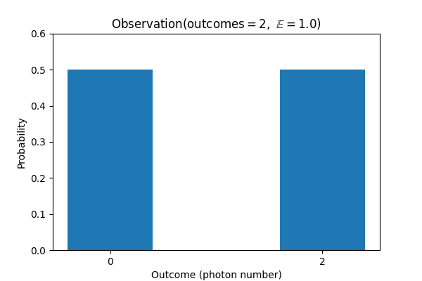
2b) Detection statistics Inspecting the states gives all possibilities, but due to generality the effective state is hidden in the canonicalization. To see the outcome statistics we can measure each port with number detector. Which should detect either 0 or 2 photons.

det = NumberDetector()
observation_port_top = det.observe(state_interfered, ports={"in": Path("bs_out0")})
observation_port_bot = det.observe(state_interfered, ports={"in": Path("bs_out0")})

VI.plot(observation_port_top)

(<Figure size 600x400 with 1 Axes>, <Axes: title={'center': '$\\mathrm{Observation}\\left(\\mathrm{outcomes}=2,\\ \\mathbb{E}=1.0\\right)$'}, xlabel='Outcome (photon number)', ylabel='Probability'>)

VI.plot(observation_port_bot)

(<Figure size 600x400 with 1 Axes>, <Axes: title={'center': '$\\mathrm{Observation}\\left(\\mathrm{outcomes}=2,\\ \\mathbb{E}=1.0\\right)$'}, xlabel='Outcome (photon number)', ylabel='Probability'>)

3) Interfering just one pulse with vacuum

Beam splitter can also work without the counterpart provided In the example below, we interfere the photon in path src_a_out with vacuum in the other port

state_interfered_single = bs(
    state_a,
    ports={
        "in0": Path("src_a_out"),
        "in1": Path("any"),
        "out0": Path("bs_out0"),
        "out1": Path("bs_out1"),
    },
).with_label("interfered_single")

VI.display_many(state_a, state_interfered_single)

4) Interfere the two states

• Join the states

• Interfere them

state_joint_dense = state_joint.to_density()

state_interfered_dense = bs(
    state_joint_dense,
    ports={
        "in0": Path("src_a_out"),
        "in1": Path("src_b_out"),
        "out0": Path("bs_out0"),
        "out1": Path("bs_out1"),
    },
).with_label("interfered")

VI.display_many(state_joint_dense, state_interfered_dense)