Envelopes¶

Overview¶

An envelope describes the temporal or spectral shape of an optical mode. All envelopes implement the abstract base class BaseEnvelope. Important concrete implementations include:

It is represented as a normalized function

\[\zeta(t) \in L^2(\mathbb{R}, \mathbb{C}),\]

which encodes the shape of the field, independent of photon number or energy.

Normalization¶

Envelopes are normalized such that

\[\langle \zeta, \zeta \rangle = 1.\]

This reflects that envelopes describe mode structure, not intensity.

Time and frequency representations¶

An envelope can be expressed in the frequency domain via

\[Z(\omega) = \int_{-\infty}^{\infty} \zeta(t)\,e^{+i\omega t}\,dt.\]

The inner product becomes

\[\langle \zeta_1, \zeta_2 \rangle = \frac{1}{2\pi} \int \overline{Z_1(\omega)} Z_2(\omega)\,d\omega.\]

Implementations provide access to both domains and may use either representation depending on context.

Gaussian envelopes¶

Gaussian envelopes form a particularly important subclass:

closed under many operations
analytically tractable
efficient to evaluate

They are parameterized by central frequency, width, temporal offset, and phase.

Many transformations preserve this structure or produce finite mixtures of Gaussian components.

Filtered and numerical envelopes¶

When analytic representations are not available, envelopes can be represented numerically.

Typical workflow:

evaluate spectrum on a grid
apply transformations pointwise
reconstruct via FFT

This provides generality at the cost of performance.

Examples¶

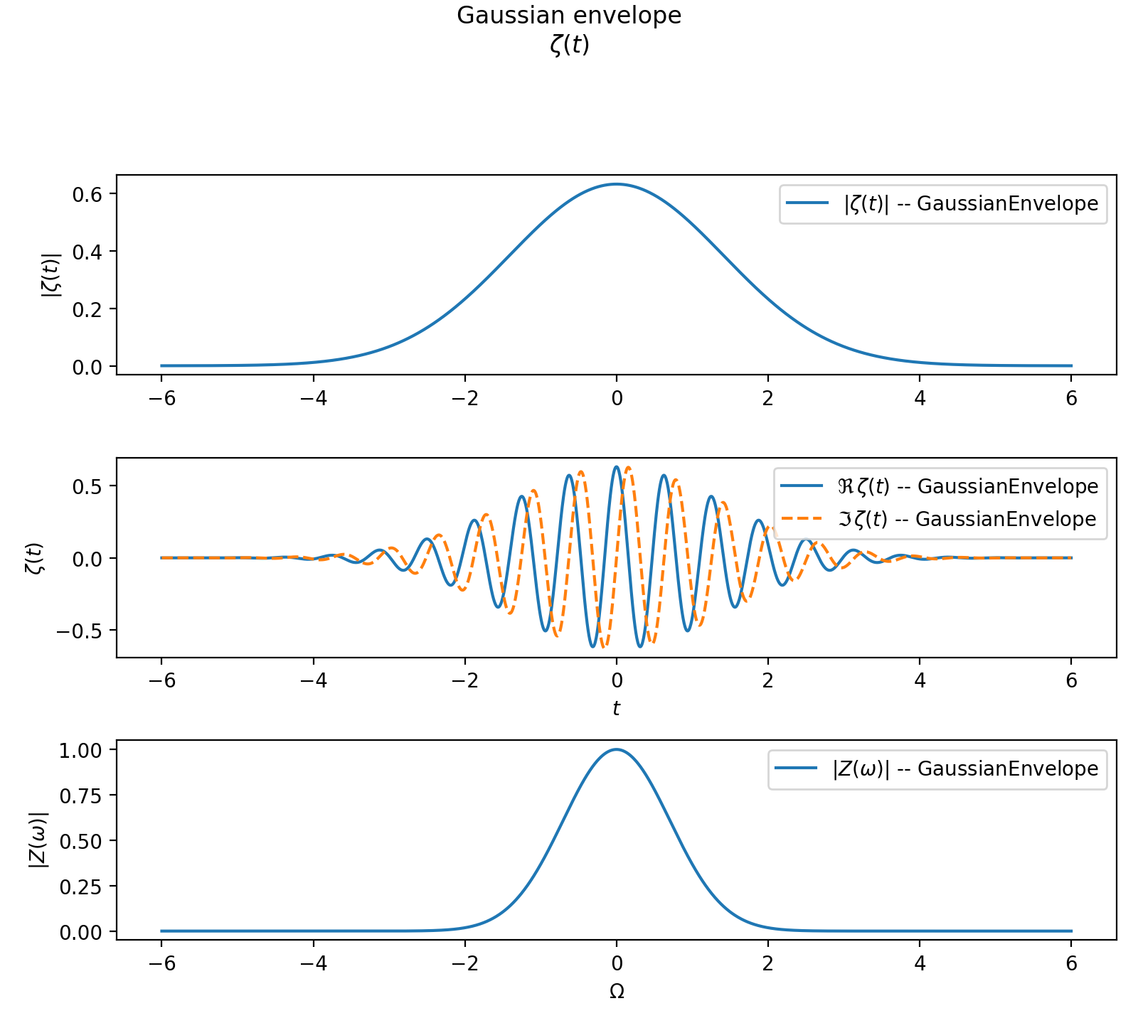
Gaussian envelope¶

import numpy as np

from symop.modes.envelopes import GaussianEnvelope
import symop.viz as viz

env = GaussianEnvelope(
    omega0=10.0,
    sigma=1.0,
    tau=0.0,
    phi0=0.0,
)


viz.plot(
    env,
    show_freq=True,
    normalize_spectrum=True,
    freq_relative=True,
    title="Gaussian envelope",
    show=False,
)

(Source code, png, hires.png, pdf)

Envelope overlap¶

from symop.modes.envelopes import GaussianEnvelope

env1 = GaussianEnvelope(omega0=10.0, sigma=1.0, tau=0.0)
env2 = GaussianEnvelope(omega0=10.0, sigma=1.0, tau=1.0)

overlap = env1.overlap(env2)

print(overlap)

(-0.7404780254568896+0.48009694530049957j)

This measures how distinguishable two temporal modes are. Identical envelopes yield an overlap of 1, while separated envelopes reduce the overlap.

Gaussian mixture (implicit)¶

Certain operations (e.g. filtering) produce mixtures of Gaussian components. These are still represented analytically when possible, without requiring numerical sampling.

Users typically do not construct mixtures manually; they arise as the result of transformations.

Design notes¶

Envelopes describe mode shape, not energy.
They are always normalized.
They support both analytic and numerical evaluation.
They form the continuous part of mode distinguishability.