Transfer functions

Overview

A transfer function (TransferBase) describes how an optical system modifies the spectral content of an envelope (typically a BaseEnvelope).

It acts multiplicatively in the frequency domain:

\[Z_{\mathrm{out}}(\omega) = H(\omega)\,Z_{\mathrm{in}}(\omega).\]

Examples

Typical transfer functions include:

• spectral filters

• phase shifts

• dispersion

• time delays

Normalization and loss

Applying a transfer produces an unnormalized result

\[Z_{\mathrm{raw}}(\omega) = H(\omega)\,Z_{\mathrm{in}}(\omega).\]

The modes subsystem enforces:

\[\eta = \langle \zeta_{\mathrm{raw}}, \zeta_{\mathrm{raw}} \rangle, \qquad \zeta_{\mathrm{out}} = \frac{\zeta_{\mathrm{raw}}}{\sqrt{\eta}}.\]

Here:

• \(\zeta_{\mathrm{out}}\) remains normalized

• \(\eta\) represents transmitted power

This separation allows loss to be handled at the quantum-state level.

Execution strategies

Gaussian-closed (analytic)

If both the envelope and transfer support analytic Gaussian representations:

• transformation is evaluated in closed form

• no sampling is required

• output is typically a Gaussian mixture

Numerical filtering

For general cases:

• spectrum is evaluated on a grid

• multiplication is performed pointwise

• result is reconstructed via FFT

This path is more general but computationally heavier.

Gaussian transfer formalism

Gaussian-compatible transfers can be expressed as

\[H(\omega) = c_0 + \sum_k c_k G_k(\omega),\]

where each \(G_k\) is a Gaussian atom.

Applying such a transfer to a Gaussian envelope yields a finite Gaussian mixture in closed form.

Structure-preserving operations

Some operations act directly on envelope parameters:

• time delay (shift in \(\tau\))

• phase shift

• frequency offset

These transformations preserve normalization and typically satisfy

\[\eta = 1.\]

Common transfer implementations include:

• GaussianBandpass

• RectBandpass

• TimeDelay

Transfers are typically applied using apply_transfer().

Examples

Gaussian band-pass filter (analytic)

import numpy as np

from symop.modes.envelopes import GaussianEnvelope
from symop.modes.transfer import GaussianBandpass
from symop.modes.transfer.apply import apply_transfer
import symop.viz as viz

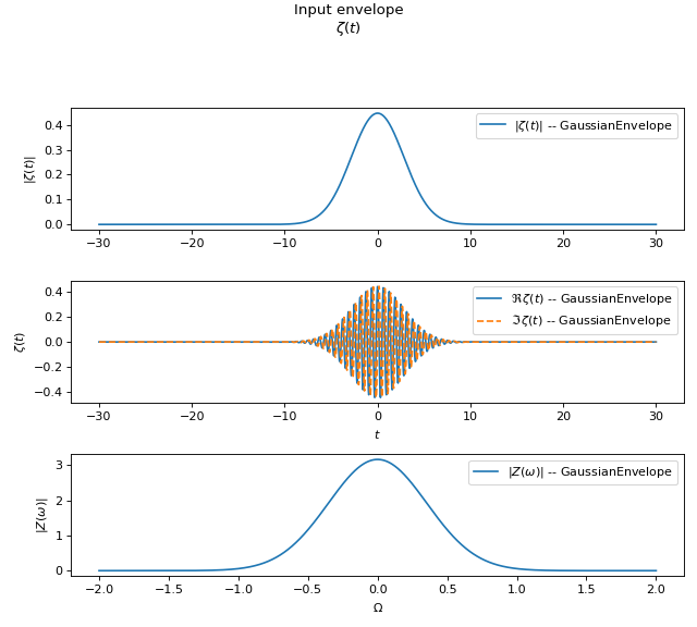
env = GaussianEnvelope(
    omega0=10.0,
    sigma=2.0,
    tau=0.0,
    phi0=0.0,
)

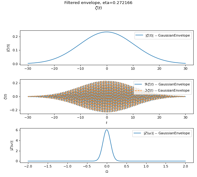
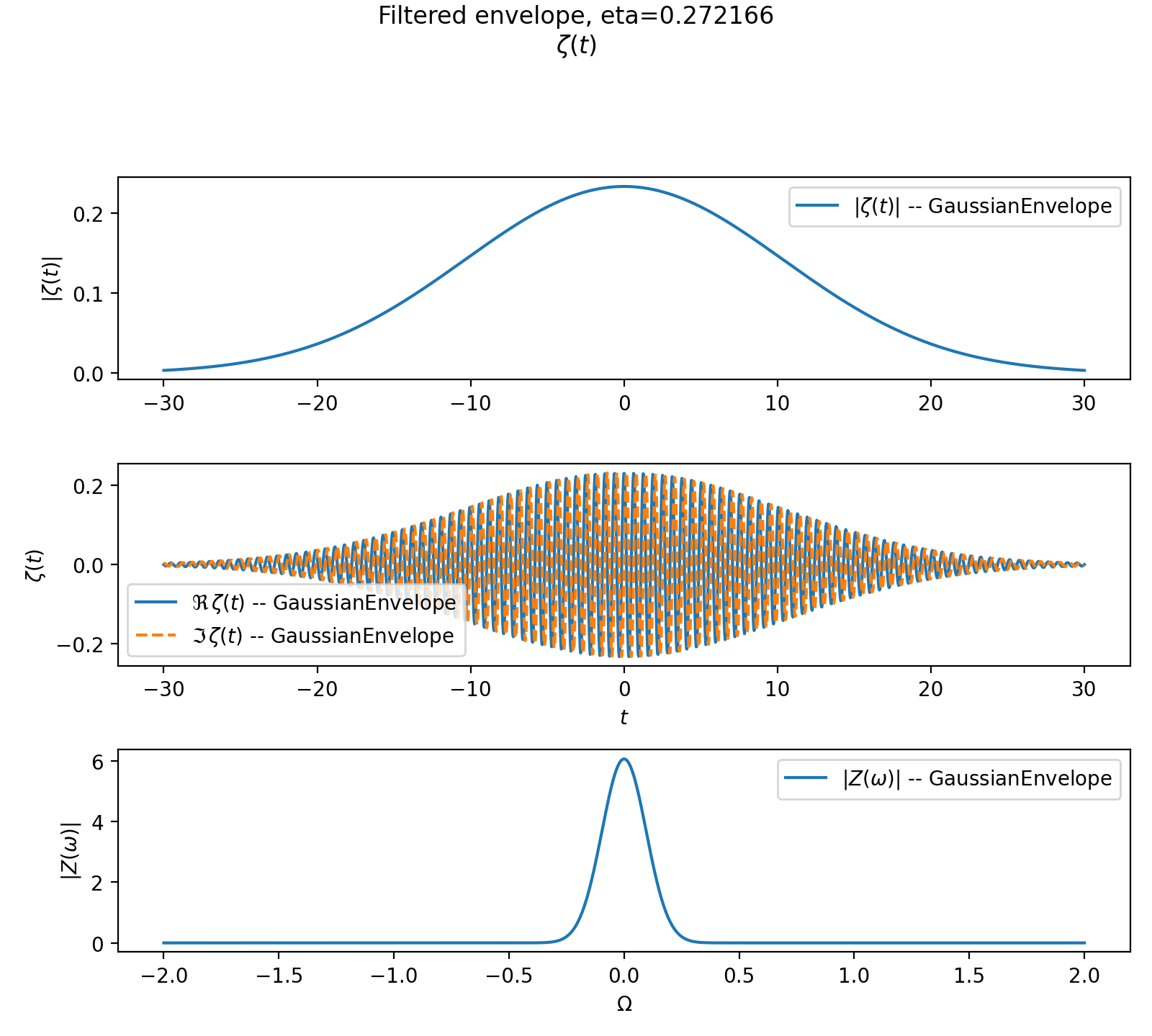
filt = GaussianBandpass(
    w0=10.0,
    sigma_w=0.1,
)

out, eta = apply_transfer(filt, env)

t = np.linspace(-30.0, 30.0, 2000)
w = np.linspace(8.0, 12.0, 2000)

viz.plot(
    env,
    t=t,
    w=w,
    title="Input envelope",
    normalize_spectrum=False,
    freq_relative=True,
    show=False,
)

viz.plot(
    out,
    t=t,
    w=w,
    title=f"Filtered envelope, eta={eta:.6f}",
    normalize_spectrum=False,
    freq_relative=True,
    show=False,
)

(Source code)

(png, hires.png, pdf)

(png, hires.png, pdf)

Expected behavior:

• output remains in the Gaussian-closed family

• \(\eta < 1\) due to filtering loss

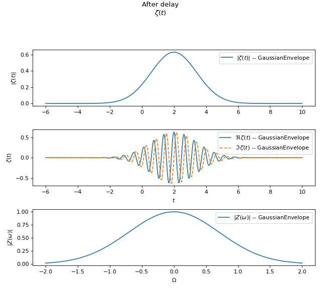
Time delay (structure-preserving)

import numpy as np

from symop.modes.envelopes import GaussianEnvelope
from symop.modes.transfer import TimeDelay
import symop.viz as viz

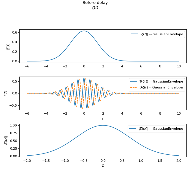
env = GaussianEnvelope(
    omega0=10.0,
    sigma=1.0,
    tau=0.0,
    phi0=0.0,
)

delay = TimeDelay(tau=2.0)

out, eta = delay.apply_to_gaussian(env)

print(out.tau, eta)

t = np.linspace(-6.0, 10.0, 2000)
w = np.linspace(8.0, 12.0, 2000)

viz.plot(
    env,
    t=t,
    w=w,
    title="Before delay",
    freq_relative=True,
    show=False,
)

viz.plot(
    out,
    t=t,
    w=w,
    title="After delay",
    freq_relative=True,
    show=False,
)

(Source code)

(png, hires.png, pdf)

(png, hires.png, pdf)

A time delay shifts the envelope in time without introducing loss:

\[\eta = 1.\]

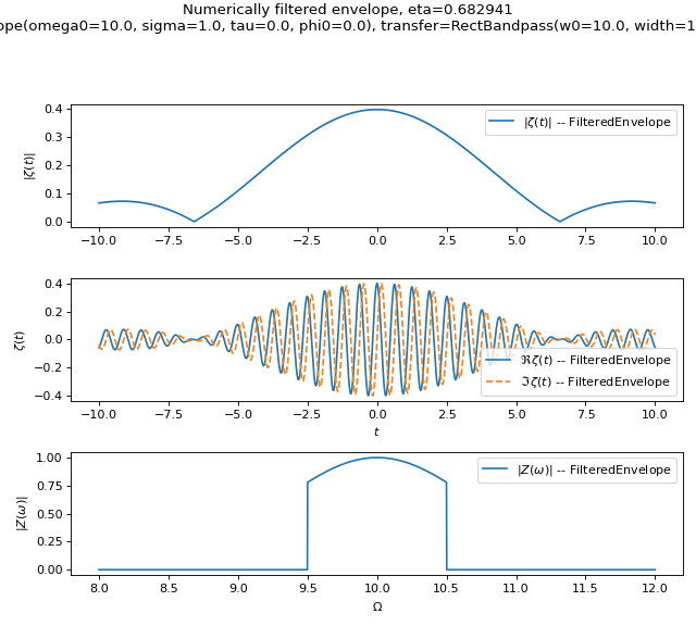
Numerical filtering fallback

import numpy as np

from symop.modes.envelopes import GaussianEnvelope
from symop.modes.transfer import RectBandpass
from symop.modes.transfer.apply import apply_transfer
import symop.viz as viz

env = GaussianEnvelope(
    omega0=10.0,
    sigma=1.0,
    tau=0.0,
    phi0=0.0,
)

filt = RectBandpass(
    w0=10.0,
    width=1.0,
)

out, eta = apply_transfer(filt, env)

print(type(out).__name__)
print(f"eta = {eta:.6f}")

t = np.linspace(-10.0, 10.0, 2000)
w = np.linspace(8.0, 12.0, 2000)

viz.plot(
    out,
    t=t,
    w=w,
    title=f"Numerically filtered envelope, eta={eta:.6f}",
    freq_relative=True,
    show=False,
)

(Source code, png, hires.png, pdf)

Expected behavior:

• output is a FilteredEnvelope

• evaluation is performed numerically rather than analytically

Design notes

• Transfers act in the frequency domain.

• They may introduce loss, captured by \(\eta\).

• Analytic and numerical paths share a common interface.

• Transfers compose algebraically.