Polarization

Overview

A Polarization label represents the polarization component of an optical mode.

In the library, polarization is modeled by a normalized Jones vector

\[\begin{split}\mathbf{v} = \begin{pmatrix} a \\ b \end{pmatrix}, \qquad \|\mathbf{v}\|_2 = 1.\end{split}\]

This representation is used to compute polarization overlaps and to provide stable mode identities for comparison, caching, and composite mode labeling.

Physical meaning

For two polarization labels \(\mathbf{v}_1\) and \(\mathbf{v}_2\), the overlap is

\[\langle \mathbf{v}_1, \mathbf{v}_2 \rangle = \mathbf{v}_1^\dagger \mathbf{v}_2.\]

This overlap contributes directly to the total overlap of composite mode labels.

Since global phase is physically irrelevant for polarization, the class canonicalizes Jones vectors so that equivalent polarizations have stable representations.

Built-in polarization states

The following common polarization labels are provided:

• Polarization.H() — horizontal

• Polarization.V() — vertical

• Polarization.D() — diagonal

• Polarization.A() — anti-diagonal

• Polarization.R() — right-circular

• Polarization.L() — left-circular

Custom linear polarizations can also be constructed by angle, and arbitrary unitary Jones transformations can be applied.

Examples

Standard polarization states

from symop.modes.labels.polarization import Polarization

h = Polarization.H()
v = Polarization.V()
d = Polarization.D()
r = Polarization.R()

print("H =", h.jones)
print("V =", v.jones)
print("D =", d.jones)
print("R =", r.jones)

Typical output:

H = ((1+0j), 0j)
V = (0j, (1+0j))
D = ((0.7071067811865476+0j), (0.7071067811865476+0j))
R = ((0.7071067811865476+0j), -0.7071067811865476j)

Polarization overlaps

from symop.modes.labels.polarization import Polarization

h = Polarization.H()
v = Polarization.V()
d = Polarization.D()

print("⟨H|H⟩ =", h.overlap(h))
print("⟨H|V⟩ =", h.overlap(v))
print("⟨H|D⟩ =", h.overlap(d))

Expected behavior:

• h.overlap(h) == 1

• h.overlap(v) == 0

• h.overlap(d) == 1 / sqrt(2)

Visualization

from symop.modes.labels.polarization import Polarization
import symop.viz as viz

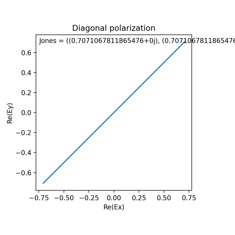
pol = Polarization.D()
viz.plot(pol, title="Diagonal polarization", show=False)

(Source code, png, hires.png, pdf)

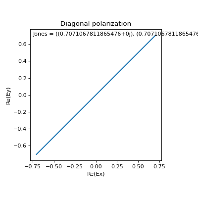
The polarization plot shows the polarization ellipse implied by the Jones vector.

Comparing linear and circular polarization

from symop.modes.labels.polarization import Polarization
import symop.viz as viz

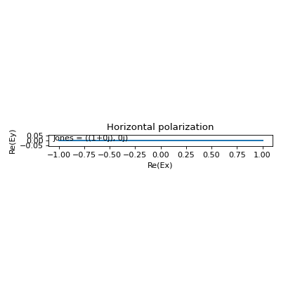
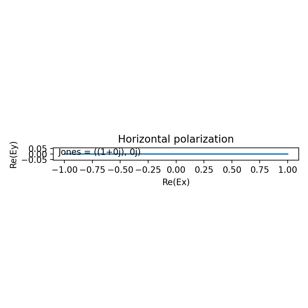
viz.plot(Polarization.H(), title="Horizontal polarization", show=False)
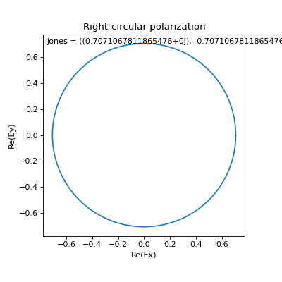
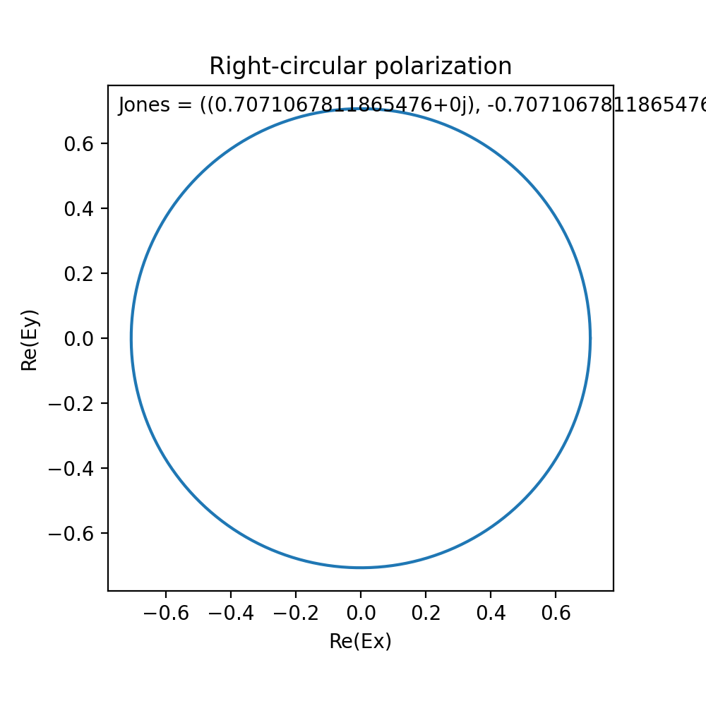
viz.plot(Polarization.R(), title="Right-circular polarization", show=False)

(Source code)

(png, hires.png, pdf)

(png, hires.png, pdf)

Linear polarizations produce degenerate ellipses aligned along a fixed axis, while circular polarizations produce circular trajectories.

Linear polarization by angle

import numpy as np

from symop.modes.labels.polarization import Polarization

pol = Polarization.linear(np.pi / 6)

print("Jones =", pol.jones)

Jones = ((0.8660254037844387+0j), (0.49999999999999994+0j))

This constructs a linear polarization at angle \(\theta = \pi/6\).

Rotation

import numpy as np

from symop.modes.labels.polarization import Polarization

h = Polarization.H()
rotated = h.rotated(np.pi / 4)

print("H =", h.jones)
print("rotated =", rotated.jones)

H = ((1+0j), 0j)
rotated = ((0.7071067811865476+0j), (0.7071067811865475+0j))

This applies a real rotation in Jones space and is useful for modeling basis changes such as half-wave plate action in a fixed convention.

Unitary transformation

import numpy as np

from symop.modes.labels.polarization import Polarization

h = Polarization.H()

U = (1 / np.sqrt(2)) * np.array([
    [1, 1],
    [1, -1],
], dtype=complex)

out = h.transformed(U)

print("input =", h.jones)
print("output =", out.jones)

input = ((1+0j), 0j)
output = ((0.7071067811865476+0j), (0.7071067811865476+0j))

This applies a Jones-space unitary transformation and returns the canonicalized output polarization.

Design notes

• Polarization labels are normalized Jones vectors.

• Global phase is removed during canonicalization.

• Overlaps are computed by the usual Jones inner product.

• Polarization is one component of a composite mode label.