Mode labels¶

Overview¶

A ModeLabel combines the three components that identify an optical mode in the library:

It represents the semantic identity of a mode and defines the overlap used when comparing modes.

Mathematically, a mode label is written as

\[m = (p, \pi, \zeta),\]

with factorized overlap

\[\langle m_1, m_2 \rangle = \langle p_1, p_2 \rangle \langle \pi_1, \pi_2 \rangle \langle \zeta_1, \zeta_2 \rangle.\]

This factorization determines whether two excitations are identical, orthogonal, or only partially overlapping.

Examples¶

Constructing a mode label¶

from symop.modes.envelopes import GaussianEnvelope
from symop.modes.labels.mode import ModeLabel
from symop.modes.labels.path import Path
from symop.modes.labels.polarization import Polarization

env = GaussianEnvelope(
    omega0=10.0,
    sigma=1.0,
    tau=0.0,
    phi0=0.0,
)

mode = ModeLabel(
    path=Path("A"),
    polarization=Polarization.H(),
    envelope=env,
)

print(mode.signature)

('mode_label', ('path', 'A'), ('pol', 1.0, 0.0, 0.0, 0.0), ('gauss', 10.0, 1.0, 0.0, 0.0))

This constructs a mode label from path, polarization, and envelope components.

Mode-label overlap¶

from symop.modes.envelopes import GaussianEnvelope
from symop.modes.labels.mode import ModeLabel
from symop.modes.labels.path import Path
from symop.modes.labels.polarization import Polarization

env1 = GaussianEnvelope(omega0=10.0, sigma=1.0, tau=0.0, phi0=0.0)
env2 = GaussianEnvelope(omega0=10.0, sigma=1.0, tau=1.0, phi0=0.0)

m1 = ModeLabel(
    path=Path("A"),
    polarization=Polarization.H(),
    envelope=env1,
)

m2 = ModeLabel(
    path=Path("A"),
    polarization=Polarization.H(),
    envelope=env2,
)

m3 = ModeLabel(
    path=Path("B"),
    polarization=Polarization.H(),
    envelope=env1,
)

print("same path/pol, shifted env =", m1.overlap(m2))
print("different path =", m1.overlap(m3))

same path/pol, shifted env = (-0.7404780254568896+0.48009694530049957j)
different path = 0j

The first overlap is generally nonzero but less than 1 because only the envelope differs. The second is exactly zero because the path labels are orthogonal.

Replacing one component¶

from symop.modes.envelopes import GaussianEnvelope
from symop.modes.labels.mode import ModeLabel
from symop.modes.labels.path import Path
from symop.modes.labels.polarization import Polarization

env = GaussianEnvelope(omega0=10.0, sigma=1.0, tau=0.0, phi0=0.0)

mode = ModeLabel(
    path=Path("A"),
    polarization=Polarization.H(),
    envelope=env,
)

mode_v = mode.with_polarization(Polarization.V())
mode_b = mode.with_path(Path("B"))

print("original =", mode.signature)
print("with V =", mode_v.signature)
print("with B =", mode_b.signature)

original = ('mode_label', ('path', 'A'), ('pol', 1.0, 0.0, 0.0, 0.0), ('gauss', 10.0, 1.0, 0.0, 0.0))
with V = ('mode_label', ('path', 'A'), ('pol', 0.0, 0.0, 1.0, 0.0), ('gauss', 10.0, 1.0, 0.0, 0.0))
with B = ('mode_label', ('path', 'B'), ('pol', 1.0, 0.0, 0.0, 0.0), ('gauss', 10.0, 1.0, 0.0, 0.0))

These helper methods make it easy to relabel one component while leaving the others unchanged.

Visualization¶

import numpy as np

from symop.modes.envelopes import GaussianEnvelope
from symop.modes.labels.mode import ModeLabel
from symop.modes.labels.path import Path
from symop.modes.labels.polarization import Polarization
import symop.viz as viz

env = GaussianEnvelope(
    omega0=10.0,
    sigma=1.0,
    tau=0.0,
    phi0=0.0,
)

mode = ModeLabel(
    path=Path("A"),
    polarization=Polarization.D(),
    envelope=env,
)

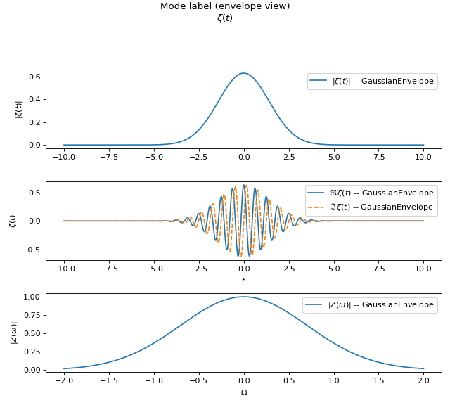
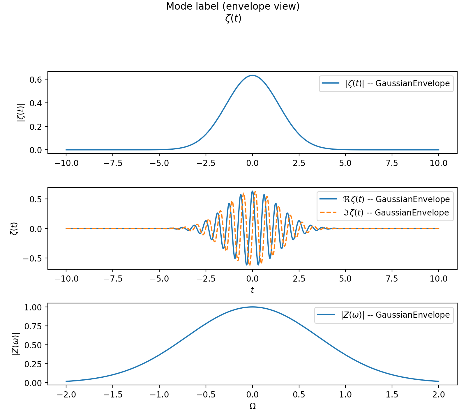
t = np.linspace(-10.0, 10.0, 2000)
w = np.linspace(8.0, 12.0, 2000)

viz.plot(
    mode,
    t=t,
    w=w,
    freq_relative=True,
    title="Mode label (envelope view)",
    show=False,
)

(Source code, png, hires.png, pdf)

Plotting a mode label delegates to the associated envelope. This is a convenient visualization of the temporal and spectral structure carried by the label.

Design notes¶

A mode label is a composite semantic identifier.
Its overlap factorizes into path, polarization, and envelope overlaps.
Plotting currently visualizes the envelope component.
Stable signatures are provided for caching and comparison.